Summary
The paper proposes Adam, a first-order optimizer that keeps exponential moving averages of the gradient () and of its elementwise square (), divides each by to remove the bias from zero initialisation, and updates (Algorithm 1). It argues that the step is approximately bounded by and invariant to gradient scale (Sec. 2.1), derives the bias correction (Sec. 3), relates Adam to AdaGrad and RMSProp (Sec. 5), and introduces AdaMax, an variant (Sec. 7.1).
Two kinds of support are offered: an regret bound for online convex optimisation (Theorem 4.1, Corollary 4.2, Appendix 10.1), and training-cost curves for logistic regression, MLPs, CNNs and a VAE ablation (Sec. 6, Figs. 1-4).
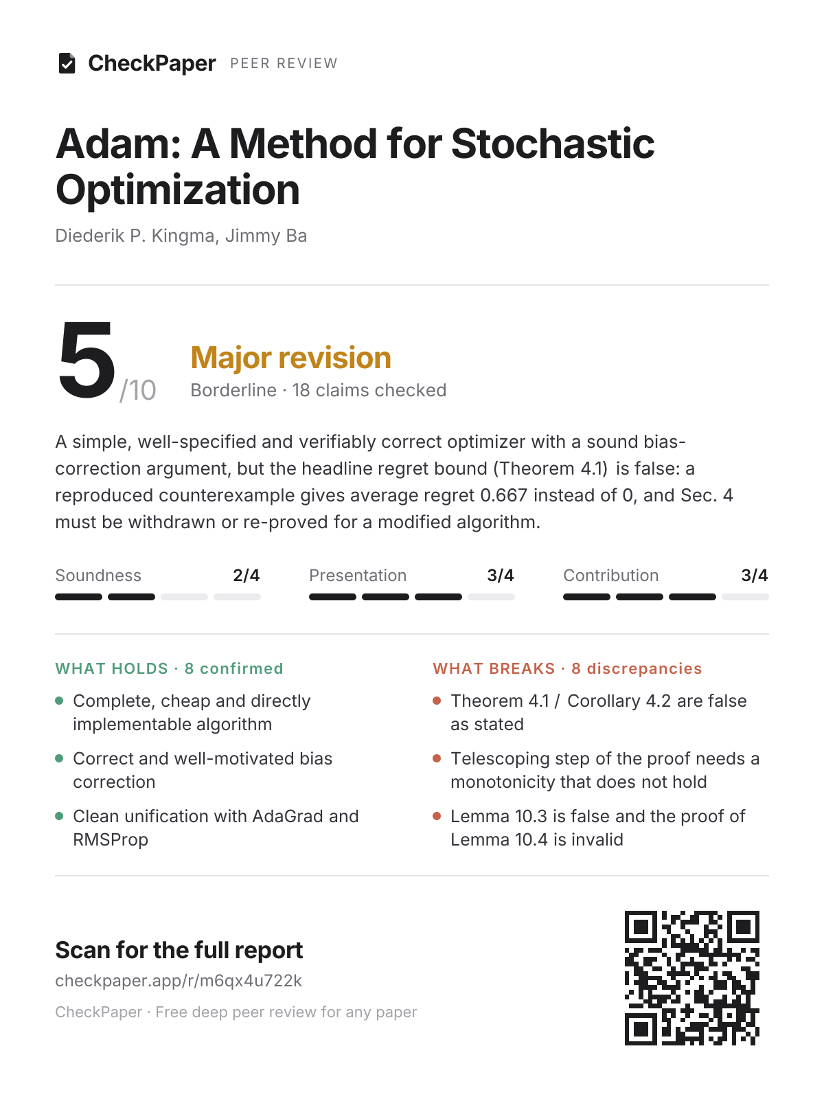
Our checks confirm the algorithmic core: the bias-correction derivation, the AdaGrad limit, the AdaMax limit, the efficient update form and the scale invariance (at ) are all correct. The convergence result is not. We reproduced an online convex problem that satisfies every hypothesis of Theorem 4.1 and on which average regret converges to 0.6667 instead of 0. We also found four independent errors in the proof. The explicit step-size bounds in Sec. 2.1 and Sec. 7.1 are exceeded by simple sequences. The experiments are single runs with undisclosed grids and no code. The overall score is one point above the rubric's cap of 4 for a main-result discrepancy. This is because the refuted result is the theorem, not the algorithm: the method and its bias correction stand independently of Sec. 4. The regret claim in the abstract and Sec. 4 does not survive.
Strengths
Complete, cheap and directly implementable algorithm
Algorithm 1 and Sec. 2 (p.2)
Algorithm 1 specifies every quantity and default (, , , ). It needs extra memory and elementwise operations only. The efficient ordering in Sec. 2 reproduces Algorithm 1 to once (check 12).
Correct and well-motivated bias correction
Sec. 3, eqs. (1)-(4) (p.3); Sec. 6.4, Fig. 4 (p.8)
Eqs. (1)-(4) are verified symbolically: . Monte Carlo gives vs. true 4.25, while the uncorrected (check 07). The correction is the paper's main technical novelty over RMSProp. Its necessity for is supported by the mechanism behind Fig. 4: uncorrected first steps grow as , i.e. 3.162α at the defaults and 10α at (check 15).
Clean unification with AdaGrad and RMSProp
Sec. 5 (p.4-5)
The limit holds symbolically for t=1..6. Numerically it matches to a relative error of 4.89e-12. Trajectories approach AdaGrad in proportion to (check 14). The contrast with RMSProp (momentum on the rescaled gradient, no bias correction) states clearly what is new.
Elegant and correct AdaMax derivation
Sec. 7.1, eqs. (6)-(12), Algorithm 2 (p.8-9)
The limit in eqs. (8)-(11) and the recursion in eq. (12) check out. The recursion equals the max formula to 1.6e-61, and the p-norm expression converges monotonically, with relative error 4.52e-9 at (check 11).
Useful practitioner intuition about step scale and invariance
Sec. 2.1 (p.2-3)
Sec. 2.1 frames as a trust-region radius and as a signal-to-noise ratio. This gives concrete guidance for setting . Invariance to scalar and diagonal gradient rescaling is exact for , with trajectories identical to 4.2e-16 (check 13). For typical gradient sequences the steps stay near (e.g. 2.66α for a spike with the defaults, check 09).
Experiments cover diverse settings and several baselines
Sec. 6.1-6.4, Figs. 1-4 (p.5-8)
The experiments span convex dense and sparse problems (MNIST and IMDB BoW logistic regression), non-convex MLPs with and without dropout, a CNN on CIFAR-10 and a VAE. They compare against SGD-Nesterov, AdaGrad, RMSProp, AdaDelta and SFO. On a synthetic sparse BoW proxy we saw the same qualitative pattern as Fig. 1 (right): adaptive methods reached final training NLL 0.0333 (Adam) and 0.0280 (AdaGrad) vs. 0.2224 for SGD-Nesterov (check 16, inconclusive as evidence about the actual figure).
Weaknesses
Theorem 4.1 / Corollary 4.2 are false as stated
major · Sec. 4, Theorem 4.1 and Corollary 4.2 (p.4); Appendix Theorem 10.5 (p.13-15)
We simulated the online problem of Reddi, Kale & Kumar (ICLR 2018): if else on . It satisfies every hypothesis (gradients ≤3, bounded iterates, , ). Adam's average regret is 0.68612, 0.66812 and 0.66692 at , converging to 2/3 rather than 0, and the iterates go to the worst point . At the regret exceeds the Theorem 4.1 right-hand side (check 01). Without projection (convex barrier instead) the value was 0.69052, and bias correction changed only in the 5th significant digit.
The claim that the regret bound is 'comparable to the best known results' (abstract, p.1) and the transfer of the Duchi et al. rate to Adam (p.4) therefore have no support. Fix: withdraw the theorem, or prove a bound for a modified algorithm. One option is to enforce a non-decreasing , e.g. by using .
Telescoping step of the proof needs a monotonicity that does not hold
major · Appendix 10.1, proof of Theorem 10.5 (p.14 to first display of p.15)
Bounding by requires every bracket to be non-negative. The assumptions do not guarantee this. On the check-01 gradient sequence, 13329 of 20000 brackets are negative (), and for a periodic spike 19980 of 20000 are negative. With iterates chosen inside the assumed bounded set, the sum exceeds the claimed bound by factors of 1.23 to 4039.54 (check 02). This is the root cause of the counterexample in check 01.
Lemma 10.3 is false and the proof of Lemma 10.4 is invalid
major · Appendix 10.1, Lemma 10.3 (p.12), Lemma 10.4 (p.13)
Lemma 10.3, , is dimensionally inconsistent: the LHS scales like and the RHS like . It fails already at the induction base: , gives LHS 1/4 > RHS 1/8. It also fails for at (4.027245195 > 4.013599479) (check 03). A valid replacement via Cauchy-Schwarz adds a factor to the second term.
The statement of Lemma 10.4 held in all 36 of our examples (max ratio 0.311). However, its proof uses , which gives 5274.4 vs. 27.819 at . The bound the proof actually reaches (with an extra and ) differs from the statement and is itself violated, e.g. 0.087994 > 0.078685 (check 04).
Constant term of the regret bound is unjustified and inconsistent
major · Appendix p.15 (last three displays); Theorem 4.1 (p.4); Theorem 10.5 (p.14)
The third term relies on . This fails for constant gradients, where . At the true sum is 2.696964e4 vs. the stated term 1.581139e4. Without the factor the bound holds. The final display on p.15 has where Theorem 4.1 has , and it is exceeded for all three tested (check 05). Theorem 4.1 also uses where the per-coordinate argument yields .
Theory analyses a different algorithm from the one proposed and tested
major · Sec. 4 (p.4) vs. Algorithm 1 (p.2); Appendix p.14; Sec. 6.1 (p.5)
Theorem 4.1 requires , a decaying and bounded iterates. Algorithm 1 uses constant and and has no projection, so boundedness is assumed about the algorithm's output rather than enforced. The proof applies the correction to a moment built with , which is biased: at for . The correct factor is (check 08). This effect is negligible for (2.7e-7), but the analysed method is not fully specified, and Sec. 6.1 never says whether was decayed. The paper should state precisely which variant each result applies to.
Explicit step-size bounds in Sec. 2.1 and for AdaMax are not upper bounds
major · Sec. 2.1 (p.2-3); Sec. 7.1, end (p.9)
Sec. 2.1 states (3.1623α at the defaults), or in the other case. Algorithm 1 with reaches 5.7812α at the defaults (the supremum tends to 7.27α). It reaches 1.8282α for (claimed ≤1) and 996.66α for , which Algorithm 1 permits. A single spike after 999 small gradients already gives 1.0846α > α (check 09).
The AdaMax claim (p.9) is exceeded too: 1.009091α at the defaults, 1.899429α at , and unbounded when (check 10). The one-hot sparse case is not the worst case, contrary to the text. Fix: state the closed-form supremum, which requires (resp. for AdaMax), and keep 'approximately bounded' as intuition.
Empirical evidence is thin and overstated
major · Sec. 1 (p.2), Sec. 6 (p.5-8), Sec. 8 (p.10), Figs. 1-3
The only protocol given is that hyper-parameters 'are searched over a dense grid' (p.5). The grids are not listed, each curve is a single run with no seeds or error bars, only training cost is reported (no held-out metrics), and no code is released. Figures 1-4 therefore cannot be regenerated (checks 16, 18).
Several sentences claim more than the figures show. p.2 says 'our method consistently outperforms other methods', while Sec. 6.3 (p.7) concedes a 'marginal improvement' over SGD on the CNN. p.6 says the performance is 'consistent with our theoretical findings in sections 2 and 4', and p.10 that 'the experiments confirm the analysis on the rate of convergence in convex problems'. Training-cost curves from single runs cannot confirm a regret bound, and that bound is false (check 01). Fix: report grids, several seeds with spread, test metrics and code, and soften these sentences.
Regret bound is vacuous for the suggested $\lambda$
minor · Sec. 4, text before Theorem 4.1 (p.4)
Taken at face value with and the defaults, the constant term is 1.58114e18 for the suggested (p.4). The bound beats the trivial only for , or at (check 06). Even a corrected theorem would need to discuss this dependence on . (Check 06 confirms at the defaults.)
Bias-correction residual $\zeta$ and $\epsilon$ effects not quantified
minor · Sec. 3, eq. (4) (p.3); Abstract; Sec. 6.3 (p.7)
Eq. (4) says 'can be kept small' under non-stationarity. With a linearly drifting second moment () and , the corrected underestimates by 32.444% at and 39.760% at (6.0% for ) (check 07). This qualifies the abstract's 'appropriate for non-stationary objectives'.
Similarly, the abstract's invariance claim holds only when . At gradient scale the trajectories deviate by 3.839e-3 (check 13), which is exactly the regime Sec. 6.3 describes, where dominates.
Notational slips and undefined symbols
minor · Sec. 2 (p.2), Sec. 3 (p.3), Sec. 5 (p.5), Sec. 7.2 (p.9)
- in the efficient form (p.2) is never defined. Equivalence to Algorithm 1 needs ; with the trajectories differ by 3.663e-3 at gradient scale (check 12).
- p.3 attributes the choice of decay rate in the derivation to ; it should be .
- p.3 says the problem arises for 'a small value of ', and p.2 speaks of small decay rates with the βs close to 1. The problem actually arises for close to 1, i.e. small (check 15).
- The AdaGrad formula on p.5 writes instead of (check 14).
- Sec. 7.2 reuses for a different decay.
Bibliographic inaccuracies
minor · References (p.10-11)
- Kingma & Welling is dated '2nd ICLR, 2013'; the 2nd ICLR was in 2014.
- Zinkevich (2003), which underpins Sec. 4, has no venue (ICML 2003).
- Tieleman & Hinton (2012) is a Coursera lecture slide cited as a technical report, so no formal specification of RMSProp is available to readers.
- Ruppert (1988) could not be located (check 17).
Questions for the authors
Given the reproduced counterexample (check 01), which satisfies every hypothesis of Theorem 4.1, which additional assumption or algorithmic change (e.g. a non-decreasing , or using ) do you propose so that an regret bound holds, and does it cover Algorithm 1 as used in Sec. 6?
Lemma 10.3 fails at T=1 for . What was the intended statement? Does the corrected version (with a factor) still give in combination with a fixed telescoping step?
In the Sec. 6.1 experiments that use , was also decayed, and with which and which bias-correction factor?
What grids were searched for each optimizer, how many seeds were run, and how much do the curves in Figs. 1-3 vary across seeds? Do the rankings hold on held-out loss or accuracy?
What value of does the efficient implementation (p.2) use, and were the experiments run with Algorithm 1 or the efficient form?
Verification
We ran 18 checks, 17 of them with rerunnable scripts, focusing on the convergence theorem and the bias correction as the requester asked.
Convergence theory: the conclusion of Theorem 4.1 is refuted by a reproduced counterexample in which (01). Four proof steps fail numerically: the telescoping step (02), Lemma 10.3 (03), the series step and constant of Lemma 10.4's proof (04), and the factor in the constant term (05). The correction is biased under decaying (08), and for the suggested the bound is vacuous at any practical horizon (06).
Bias correction and algebra: the derivation is correct (07), and so are the AdaGrad limit (14), the AdaMax limit (11), the efficient form given the right (12), scale invariance at (13) and the large uncorrected steps for (15). The explicit step-size bounds of Sec. 2.1 (09) and Sec. 7.1 (10) are exceeded.
Experiments and references: the figures could not be regenerated (no code or data); a sparse logistic-regression proxy was only qualitatively consistent (16, inconclusive; 18, not checkable). 22 of 23 references were located (17).
Theorem 4.1 / Corollary 4.2: under bounded gradients and iterates, gamma<1, alpha_t=alpha/sqrt(t), beta1,t=beta1*lambda^(t-1), R(T)=O(sqrt(T)) and R(T)/T -> 0DiscrepancySection 4, Theorem 4.1 and Corollary 4.2 (p.4); Appendix Theorem 10.5 (p.13-15)
All hypotheses hold (gradients <=3, iterates in [0.47,1.0] (A) / [0.47,1.15] (B), gamma=0<1). Theorem predicts R(T)/T -> 0; obtained R(T)/T = 0.68612 (T=1e3), 0.67165 (1e4), 0.66812 (1e5), 0.66712 (1e6), 0.66692 (3e6) for projected bias-corrected Adam, converging to 2(C-2)/3=0.6667; unprojected+barrier 0.69052 at T=3e6. Iterates converge to x=+1 (worst point) instead of x*=-1. At T=3e6, R(T)=2.00e6 exceeds the Theorem 4.1 RHS 1.40e5, so the stated inequality is violated, not just the rate. Bias correction changes R(T) only in the 5th significant digit here.
script: 01_regret_counterexample.pySimulated Adam (Algorithm 1 moments, alpha_t=0.5/sqrt(t), beta1=0 so beta1,t=0 and gamma=0, beta2=1/(1+C^2)=0.1, eps=0) on the Reddi-Kale-Kumar (2018) online problem f_t(x)=3x if t mod 3==1 else -x, X=[-1,1]; (A) projected onto X, (B) unprojected with a shared convex barrier 10*max(0,|x|-1)^2; with and without bias correction; T up to 3e6. Evaluated the Theorem 4.1 RHS (d=1, G_inf=3, D=D_inf=2, v_hat_T<=G_inf^2).
Proof step: sum_t (theta_t-theta*)^2 (sqrt(v_hat_t)/alpha_t - sqrt(v_hat_{t-1})/alpha_{t-1}) <= D_inf^2 sqrt(T v_hat_T)/alpha, which needs sqrt(t v_hat_t) non-decreasingDiscrepancyAppendix 10.1, proof of Theorem 10.5 (p.14, regret decomposition) to first display of p.15
Negative brackets are common: e.g. 13329/20000 (beta2=0.9) and 12885/20000 (beta2=0.999) on the check-01 sequence (3,-1,-1,...); 19980/20000 for a periodic spike with beta2=0.999. The weighted sum exceeds the claimed bound D_inf^2 sqrt(T v_hat_T)/alpha by factors 1.23 to 4039.54 (claimed ratio <= 1, tolerance 1e-9). The telescoping step therefore does not follow from the stated assumptions; this is the gap identified by Reddi et al. (2018). Caveat: the theta_t sequence is chosen adversarially within the assumed bounded set rather than generated by Adam; check 01 shows the conclusion itself fails for Adam-generated iterates.
script: 02_telescoping_gap.pyRan the bias-corrected v_hat recursion (beta2 in {0.9, 0.999}, T=20000) on three gradient sequences, counted negative brackets sqrt(t v_hat_t)-sqrt((t-1)v_hat_{t-1}), and evaluated the weighted sum with (theta_t-theta*)^2 chosen in {0, D_inf^2} (theta*=0, theta_t in {0,D_inf}, so |theta_m-theta_n|<=D_inf holds) against the claimed bound
Lemma 10.3: sum_{t=1}^T sqrt(g_{t,i}^2/t) <= 2 G_inf ||g_{1:T,i}||_2 for |g_t|<=G_infDiscrepancyAppendix 10.1, Lemma 10.3 and inductive proof (p.12)
(i) T=1, G_inf=1/4, g_1=1/4: LHS=1/4 > RHS=1/8, so the base case of the induction fails. (ii) g_t=G_inf/sqrt(t) with G_inf=1 (all |g_t|<=1): first failure at T=31, LHS=4.027245195 > RHS=4.013599479; with G_inf=1.5 first failure at T=4550 (13.50031209 > 13.50015605). (iii) Rescaling g by c multiplies the LHS by c and the RHS by c^2: with c=0.1 on g_t=1/sqrt(t), t<=10: LHS=0.29289683 > RHS=0.034228457. The lemma is dimensionally inconsistent and false as stated; a valid replacement is Cauchy-Schwarz, sum |g_t|/sqrt(t) <= ||g_{1:T}||_2 sqrt(H_T) = O(||g|| sqrt(log T)), which would add a log factor to the second term of Theorem 4.1. (A sub-check (iv) on the final rearrangement in the proof was not diagnostic and is not used.)
script: 03_lemma103.pyExact counterexamples with fractions/mpmath (40 digits): base case T=1; sequence g_t=G_inf/sqrt(t); gradient rescaling
Lemma 10.4: sum_t m_hat_{t,i}^2/sqrt(t v_hat_{t,i}) <= 2/((1-gamma) sqrt(1-beta2)) ||g_{1:T,i}||2; proof ends at 2 G_inf/((1-gamma)^2 sqrt(1-beta2)) ||g{1:T,i}||2 and uses sum{j=0}^{T-t} t gamma^j <= 1/(1-gamma)^2DiscrepancyAppendix 10.1, Lemma 10.4 statement and proof (p.13)
The lemma statement held in all 36 examples (max LHS/stated bound = 0.311104), so the statement itself was not refuted. But (a) the series step used in the proof is false: at t=1000, T=2000, sum_j t*gamma^j = 5274.4 vs claimed <= 1/(1-gamma)^2 = 27.819 (beta1=0.9, beta2=0.999, gamma=0.81041), and 51521 vs 2654.4 for beta1=0.99; (b) the bound actually reached at the end of the proof (with G_inf and (1-gamma)^2) is violated in 5 examples, e.g. beta1=0.9, beta2=0.999, constant gradient 1e-3: LHS 0.087994 > 0.078685; beta1=0, beta2=0.9, gradient 1e-3: 0.087994 > 0.00028284. Statement and proof also disagree on the constant. The proof does not establish the lemma as used in Theorem 4.1.
script: 04_lemma104.pyRan Algorithm 1 moments (constant beta1, eps=0) for T=2000 on constant, random-sign, sparse (every 100th step) and exponentially growing gradients at scales 1e-3, 1, 1e3, for (beta1,beta2) in {(0,0.9),(0.9,0.999),(0.99,0.999)}; compared the sum with the stated bound and the proof-final bound; evaluated the series inequality at t=1000
Third (constant) term of Theorem 4.1: (D_inf^2/(2alpha)) sum_t beta1,t/(1-beta1,t) sqrt(t v_hat_t) <= D_inf^2 G_inf sqrt(1-beta2)/(2alpha(1-beta1)(1-lambda)^2); p.15 final display has 2 alpha beta1 (1-lambda)^2 insteadDiscrepancyAppendix p.15 (last three displays) vs Theorem 4.1 (p.4) and Theorem 10.5 (p.14)
lambda=0.9: LHS=2.696964e+04 exceeds the theorem term 1.581139e+04 (ratio 1.71). The p.15 final-line variant (beta1 instead of 1-beta1) is exceeded for all three lambdas (e.g. lambda=0.999: 2.266090e+07 > 1.756821e+07). Without the sqrt(1-beta2)=0.0316 factor the bound holds in all cases (e.g. 2.70e4 <= 5.00e5), and the sub-steps sum lambda^(t-1)sqrt(t) <= 1/(1-lambda)^2 (28.56 <= 100 at lambda=0.9) and sqrt(v_hat_t) <= ||g_1:t||_2 (max ratio 1.000000) are correct. Conclusion: the sqrt(1-beta2) factor in the third term is unjustified (the proof would need sqrt(v_hat_t) <= G_inf sqrt(1-beta2), false for constant gradients where v_hat_t=G_inf^2), and the constant in the p.15 final line differs from the theorem statement.
script: 05_constant_term.pyConstant gradient g_t=G_inf=1 (bias-corrected v_hat_t=1 exactly), beta1=0.9, beta2=0.999, alpha=1e-3, D_inf=1, beta1,t=0.9 lambda^(t-1); summed LHS to convergence for lambda in {0.9,0.99,0.999}; compared with the theorem term, the p.15 final-line term and the bound without sqrt(1-beta2); also checked sum lambda^(t-1) sqrt(t) <= 1/(1-lambda)^2 and sqrt(v_hat_t)<=||g_1:t||_2
Default hyper-parameters satisfy gamma=beta1^2/sqrt(beta2)<1, and with the suggested lambda (e.g. 1-1e-8) Theorem 4.1 gives an O(sqrt(T)) guaranteeConfirmedSection 4, text before Theorem 4.1 (p.4); Algorithm 1 defaults (p.2)
gamma=0.8104053<1 at defaults (confirmed, exact). Taking the bound at face value: sqrt(T) coefficients 5000.0 + 16.7148, constant term 1.58114e+18 for lambda=1-1e-8 (1.58114e+8 for lambda=0.999, 15811.4 for lambda=0.9). The bound is below the trivial regret TGD only for T >= 1.581e+18 (lambda=1-1e-8), 2.35e+8 (lambda=0.999), 2.52e+7 (lambda=0.9). So with the value of lambda suggested on p.4 the O(sqrt(T)) guarantee is vacuous for any practical horizon; this is a presentation/relevance issue additional to checks 01-05.
script: 06_bound_vacuity.pympmath (50 digits): gamma at defaults; each term of the Thm 4.1 bound with G=G_inf=D=D_inf=1, d=1, alpha=1e-3, beta1=0.9, beta2=0.999, worst case v_hat_T=1, ||g_1:T||=sqrt(T); bisection for the smallest T where the bound drops below the trivial bound TGD
Bias correction: v_t=(1-beta2) sum beta2^(t-i) g_i^2 (eq. 1); E[v_t]=Eg^2+zeta, zeta=0 for stationary moments (eqs. 2-4); dividing by (1-beta2^t) (analogously 1-beta1^t for m_t) removes the initialisation biasConfirmedSection 3, eqs. (1)-(4) (p.3); Algorithm 1 (p.2)
(1-b) sum_{i=1}^t b^(t-i) - (1-b^t) simplifies to 0; recursion equals eq. (1) for t=1..8. MC: E[v_hat_1]=4.2599 +/- 0.0135 vs true 4.25; E[v_hat_50]=4.2454 +/- 0.0019; E[m_hat_1]=0.5003 +/- 0.0045 vs 0.5; all |z| <= 2.44 over 10 estimates (tolerance |z|<4), while uncorrected E[v_1]=0.00426 (1000x too small). Caveat for eq. (4): zeta is not small in general for beta2=0.999: with E[g_t^2]=1+0.02t the bias-corrected v_hat underestimates E[g_t^2] by 32.444% at t=100 and 39.760% at t=1000 (6.0% for beta2=0.9); the paper only says zeta can be kept small, and the text attributes this to the choice of beta1 (should be beta2).
script: 07_bias_correction.pysympy: symbolic geometric sum for symbolic t and unrolled recursion for t=1..8; Monte Carlo (seed 0, 200k replicates, g~N(0.5, 2^2), beta1=0.9, beta2=0.999) of E[m_hat_t], E[v_hat_t] at t in {1,2,5,10,50} with SE; exact expectation for a drifting second moment E[g_t^2]=1+0.02t
The convergence proof applies bias correction 1-beta1^t to a first moment built with time-varying beta1,t=beta1*lambda^(t-1)DiscrepancyAppendix p.14, update-rule rewrite in proof of Theorem 10.5; Section 3 (p.3); Theorem 4.1 (p.4)
With the correction 1-beta1^t the first-moment estimate is no longer unbiased under decaying beta1,t: m_hat/E[g] = 1.426316 (t=2), 1.939168 (t=5), 1.530668 (t=10) for lambda=0.9; max deviation 0.1948 for lambda=0.99; 2.729e-07 for lambda=1-1e-8 (negligible). The correct correction is 1-prod_{k<=t} beta1,k. The effect is only material for lambda well below 1, but it means the algorithm analysed in Section 4 is not exactly specified (Algorithm 1 has constant beta1 and alpha).
script: 08_varying_beta1.pyRan m_t=beta1,t m_{t-1}+(1-beta1,t) g_t with g_t=1 (so m_t equals the weight sum W_t=1-prod beta1,k) for beta1=0.9 and lambda in {0.9, 0.99, 1-1e-8}; compared m_t/(1-beta1^t) with the true mean 1
With eps=0, |Delta_t| <= alpha(1-beta1)/sqrt(1-beta2) if (1-beta1)>sqrt(1-beta2), else |Delta_t| <= alpha; first case only under the most severe sparsityDiscrepancySection 2.1 (p.2-3)
Defaults (case 1, claimed <= 3.1623): extremal sequence gives |Delta_t|/alpha = 5.7812 at t=1000 (closed-form sup 5.7812; t->inf limit 7.27). Case 2 (claimed <= 1): beta1=0.99, beta2=0.999 gives 1.8282 at t=1000; beta1=0.9, beta2=0.99 gives 2.3452, and a single gradient spike after 999 small gradients already gives 1.0846 > 1; beta1=0.9, beta2=0.8 (beta1^2>beta2, allowed by Algorithm 1) gives 996.6555, i.e. no bound at all. 10 of 12 extremal cases violate the stated bound (tolerance 1e-9). The extremal sequences require geometrically growing gradients, so the bound is approximately right for typical sequences (spike case with defaults 2.6583 < 3.1623), but it is not an upper bound, and the one-hot sparse case is not the worst case. A correct bound is the closed form printed by the script, which requires beta1^2 < beta2.
script: 09_step_bound.pyDerived the Cauchy-Schwarz supremum of |m_hat_t/sqrt(v_hat_t)| and ran Algorithm 1 (eps=0) on the extremal sequence g_i=(beta1/beta2)^(t-i), on a spike after small gradients (999 x 1e-2 then 1) and on the one-hot sparse case, for (beta1,beta2) in {(0.9,0.999),(0.99,0.999),(0.9,0.99),(0.9,0.8)}, t in {10,100,1000}
AdaMax: magnitude of parameter updates is bounded, |Delta_t| <= alphaDiscrepancySection 7.1, end (p.9); Algorithm 2 (p.9)
max_t |Delta_t|/alpha = 1.009091 at defaults (beta2=0.999), 1.099999 (beta2=0.99), 1.899429 (beta2=0.95), and 3.77e7 for beta2=0.8 < beta1 (unbounded growth); simulation matches the closed form to 1e-6. Claimed <= 1 (tolerance 1e-12). The correct bound is (1-beta1)/(1-beta1/beta2) for beta1<beta2, so the claim is nearly right at defaults (0.9% excess) but false in general, and there is no bound when beta1 >= beta2. A first version of the script used growing gradients by mistake (ratio <= 1); corrected and rerun.
script: 10_adamax_bound.pyRan Algorithm 2 on gradients decaying at rate beta2 (g_t = beta2^t, which makes all terms of u_t tie) for t<=150, beta1=0.9, beta2 in {0.999, 0.99, 0.95, 0.8}; compared with closed form (1-b1)(1-(b1/b2)^t)/((1-b1/b2)(1-b1^t))
AdaMax derivation: lim_{p->inf} ((1-beta2^p) sum beta2^(p(t-i))|g_i|^p)^(1/p) = max_i beta2^(t-i)|g_i| (eqs. 8-11), equal to u_t=max(beta2 u_{t-1},|g_t|), u_0=0 (eq. 12)ConfirmedSection 7.1, eqs. (6)-(12) (p.8-9); Algorithm 2
Recursion equals the max formula to 1.56e-61 (tolerance 1e-50). Relative error of the p-norm expression decreases monotonically to the max: e.g. beta2=0.999: 0.3, 0.0232, 0.000458, 4.52e-9 at p=10,100,1e3,1e4 (max over sequences at p=1e4: 4.52e-9). Eqs. (8)-(12) are correct; the absence of bias correction for u_t is consistent with u_1=|g_1|.
script: 11_adamax_limit.pympmath at 60 digits, 10 random sequences of length 20 (beta2=0.999 and 0.9): p-norm expression at p=10,100,1e3,1e4 vs max formula; recursion vs max formula
Efficient ordering alpha_t=alpha sqrt(1-beta2^t)/(1-beta1^t), theta_t=theta_{t-1}-alpha_t m_t/(sqrt(v_t)+eps_hat) is equivalent to Algorithm 1ConfirmedSection 2, last paragraph (p.2)
Equivalent to rounding error for eps=0 (max |diff| 1.110e-16 / 3.331e-16) and for eps_hat=epssqrt(1-beta2^t) (2.220e-16 / 1.110e-16), tolerance 1e-12. With eps_hat=eps (the natural reading, since eps_hat is never defined) the trajectories differ: 3.857e-09 at gradient scale 1 but 3.663e-03 at scale 1e-6 (after 1000 steps with alpha=1e-3). The paper should state eps_hat = epssqrt(1-beta2^t) (minor clarity issue).
script: 12_efficient_form.pyRan Algorithm 1 and the efficient form side by side for 1000 steps on a noisy diagonal quadratic (d=10, seed 0), gradient scales 1 and 1e-6, with eps=0, eps_hat=eps=1e-8 and eps_hat=eps*sqrt(1-beta2^t)
Adam is invariant to (diagonal) rescaling of the gradientsConfirmedAbstract (p.1); Section 2.1 last sentences (p.3)
eps=0: trajectories identical to rounding (max |diff| <= 4.163e-16, tolerance 1e-10) for scalar and diagonal rescaling. With the default eps=1e-8 invariance holds only when |g| >> eps: max |diff| 3.858e-09 (c=1e3), 3.858e-06 (c=1e-3), 3.839e-03 (c=1e-6), 2.413e-01 (c=1e-8). The claim is correct as stated with the eps=0 assumption made in Section 2.1; the abstract omits this qualification, which matters for the Section 6.3 observation that eps dominates when v_hat vanishes.
script: 13_scale_invariance.pyAlgorithm 1 on a noisy diagonal quadratic (d=5, seed 0, 2000 steps, alpha=1e-3) with gradients multiplied by c in {1e-8,1e-6,1e-3,1e3} and by diag(1e-6,1e-3,1,1e3,1e6); max deviation of the theta trajectory from c=1, for eps=0 and eps=1e-8
lim_{beta2->1} v_hat_t = t^-1 sum_i g_i^2; Adam with beta1=0, (1-beta2)->0, alpha_t=alpha/sqrt(t) reduces to AdaGrad; without bias correction the update blows upConfirmedSection 5, AdaGrad paragraph (p.5)
Symbolic limit equals the mean of g_i^2 for t=1..6. t=50: v_hat=0.846800729488511 vs mean 0.846800729484373 (rel. diff 4.89e-12, tolerance 1e-9). Trajectory gap to AdaGrad scales with 1-beta2: 3.696e-02 (beta2=0.99), 3.695e-04 (0.9999), 3.692e-08 (1-1e-8, tolerance 1e-6). Without bias correction the first step is alpha/sqrt(1-beta2), e.g. 1000 alpha at beta2=0.999999, diverging as beta2->1. Minor: the AdaGrad formula on p.5 writes sum_{i=1}^t g_t^2 (index should be g_i).
script: 14_adagrad_limit.pysympy limit b->1 for t=1..6 with symbolic g_i; mpmath (40 digits) at t=50, beta2=1-1e-12; 200-step trajectories on a noisy 1-D quadratic (seed 1) for limiting Adam vs AdaGrad; uncorrected first-step factor 1/sqrt(1-beta2)
Without bias correction, beta2 close to 1 leads to much larger initial steps (motivating Fig. 4); p.3 phrases this as the case of a small value of beta2ConfirmedSection 3 last paragraph (p.3); Section 5 RMSProp paragraph (p.5); Section 6.4 and Figure 4 (p.8)
Uncorrected first step = (1-beta1)/sqrt(1-beta2): with beta1=0.9 it is 0.316, 1.000, 3.162, 10.000 alpha for beta2=0.9, 0.99, 0.999, 0.9999 (median max over 100 dense steps 0.514, 1.301, 4.085, 12.912) while the corrected step stays at 1.000 alpha; monotone in beta2 in all 4 settings. This supports the mechanism behind Section 6.4/Fig. 4. The p.3 sentence says the problem arises for a small value of beta2; it arises for beta2 close to 1 (small 1-beta2), so the wording is inverted (minor). Also, the sparse beta1=0 bias-corrected case reaches a median max of 5.232 alpha, above the approximate alpha bound of Section 2.1 (consistent with check 09).
script: 15_uncorrected_steps.pyAlgorithm 1 moments with/without bias correction (eps=1e-8) on 1000 independent coordinates (seed 0), dense N(0,1) and sparse (5%) gradients, beta1 in {0,0.9}, beta2 in {0.9,0.99,0.999,0.9999}; median of first-step and max-over-100-steps |Delta_t|/alpha
Adam matches AdaGrad on sparse (IMDB BoW) logistic regression and beats SGD-Nesterov (Fig. 1); outperforms other methods on MLPs and CNNs (Figs. 2-3)InconclusiveSection 6.1-6.3, Figures 1-3 (p.5-7)
Best final training NLL: Adam 0.0333 (alpha=3), AdaGrad 0.0280 (alpha=3), SGD-Nesterov 0.2224 (alpha=100). The qualitative pattern of Fig. 1 right (adaptive methods ~ each other and far ahead of SGD-Nesterov on sparse features) is reproduced on this proxy, but this is not evidence about the specific curves in Figures 1-3, which report single runs of training cost without error bars. The MLP/CNN/VAE results (Figs. 2-4) were not examined.
script: 16_sparse_logreg.pyNo code, data pipeline, numeric values, seeds or hyper-parameter grids are provided, so Figures 1-3 cannot be regenerated. Qualitative proxy only: synthetic sparse bag-of-words logistic regression (N=20000, D=10000, Zipf frequencies, 29.5 nonzeros/doc, seed 0), minibatch 128, 10 epochs, alpha/sqrt(t) decay for Adam and SGD-Nesterov (momentum 0.9), AdaGrad with constant alpha; 5-point grid per method with interior optimum
Bibliography entries exist and are cited correctly; load-bearing references (Duchi et al. 2011, Zinkevich 2003, Tieleman & Hinton 2012, Sutskever et al. 2013) support the statements they are cited forConfirmedReferences (p.10-11); citations on p.1, p.4, p.5
22 of 23 references resolved to the cited work (Crossref DOI, arXiv abstract page, or canonical JMLR/PMLR/NeurIPS/ACL/ICML/AAAI pages); Ruppert 1988 (Cornell technical report) could not be located online (not_checkable, but widely cited). Citation-detail issues: Kingma & Welling listed as 2nd ICLR 2013; arXiv 1312.6114 was submitted 20 Dec 2013 and the 2nd ICLR took place in 2014. Zinkevich 2003 has no venue (it is ICML 2003, AAAI library ICML03-120). Tieleman & Hinton 2012 is cited as a Technical report; it is a Coursera lecture slide (Lecture 6e, rmsprop found in the slide text). Support: Sutskever et al. 2013 PDF states that reducing the momentum coefficient allows for finer convergence (supports p.4); Duchi et al. 2011 give the O(log d) sparse-feature example (supports the AdaGrad part of p.4, while the transfer to Adam rests on Theorem 4.1). No reference was found to be non-existent.
script: 17_refs.pytools/check_refs.py (Crossref/arXiv; arXiv API returned HTTP 406) then work/verify/17_refs.py (arXiv abstract pages + Crossref title/author query), 17b_refs_canonical.py (publisher pages/PDFs for no-DOI venues), 17c_refs_support.py (text search in the cited PDFs)
Adam outperforms or matches other optimisers on MLPs (Fig. 2), CNNs (Fig. 3) and the VAE bias-correction ablation (Fig. 4)Not checkableSections 6.2-6.4, Figures 2-4 (p.6-8)
Regenerating these figures would require the training code, preprocessing (e.g. CIFAR-10 whitening, IMDB BoW features), the searched grids and seeds; reproducing CNN/VAE training at the reported scale is also beyond this CPU-only budget. The mechanism behind Fig. 4 was checked separately (check 15).
None possible: no released code (request.json code_url null), no numeric values behind the curves, hyper-parameter grids described only as a dense grid, single runs, no seeds
References
23 references checked
- Kingma & Welling 2013, Auto-Encoding Variational Bayes, 'The 2nd International Conference on Learning Representations (ICLR), 2013'
Year/venue mismatch: the 2nd ICLR took place in 2014; arXiv:1312.6114 was submitted 20 Dec 2013 (verified on arxiv.org). Should read ICLR 2014 (or arXiv 2013).
- Zinkevich 2003, Online convex programming and generalized infinitesimal gradient ascent
Incomplete entry: no venue given. The work is ICML 2003 (found at cdn.aaai.org/ICML/2003/ICML03-120.pdf). Load-bearing for Section 4; content matches the citation (online convex programming framework, regret).
- Tieleman & Hinton 2012, Lecture 6.5 - RMSProp, COURSERA, 'Technical report'
Mis-typed as a technical report: it is an unpublished Coursera lecture slide deck (Lecture 6e, 'rmsprop: Divide the gradient by a running average of its recent magnitude'). Content supports the RMSProp description, but readers cannot consult a formal specification (e.g. no bias correction, no epsilon).
- Ruppert 1988, Efficient estimations from a slowly convergent Robbins-Monro process, Cornell technical report
Could not be located online (Crossref returned unrelated works); existence not verified, though it is a widely cited technical report. Not load-bearing (cited for Polyak-Ruppert averaging in Section 7.2).
- Duchi et al. 2011 (cited on p.4 for O(log d sqrt(T)) vs O(sqrt(dT)))
The reference supports the claim for AdaGrad (their Section 1.2 example gives an O(log d) factor for sparse features), but the paper states that 'their results ... also apply to Adam', which depends on Theorem 4.1; checks 01-05 show that theorem and its proof do not hold as stated, so this transfer is unsupported.
Suggestions
Replace Sec. 4 and Appendix 10.1 with a correct result. Either restrict the claim to a modified algorithm whose effective step is non-increasing, and prove it, or remove the regret claim from the abstract and conclusion.
Correct Lemma 10.3 (e.g. via Cauchy-Schwarz, accepting a factor), align the statement and proof of Lemma 10.4, and make the constants in Theorems 4.1 and 10.5 and the final display on p.15 agree ( vs. , vs. , the factor).
If decays, use the bias correction and state explicitly which algorithm variant each theoretical and empirical result refers to.
Replace the inequalities in Sec. 2.1 and Sec. 7.1 by the exact supremum of (resp. ), state the needed condition (resp. ), and present 'approximately bounded by α' as typical-case intuition.
Release code. List the hyper-parameter grids per optimizer, report several seeds with confidence bands and held-out metrics, and add wall-clock comparisons.
Soften 'consistently outperforms' (p.2) and 'the experiments confirm the analysis on the rate of convergence' (p.10) to match Fig. 3 and the status of the theory.
Define in the efficient form, and qualify the invariance claim in the abstract with .
Quantify in eq. (4) for a simple drift model and discuss the trade-off in the choice of for non-stationary objectives. Fix the slips on p.2-3 and the index typo on p.5.
Update the bibliography: Kingma & Welling (ICLR 2014), Zinkevich (ICML 2003), Tieleman & Hinton (lecture slides).
Scope of this review
The arXiv source contains no LaTeX for the paper body (arxiv.tex only includes a PDF), so equations were read from the PDF text and checked against the page layout. No code repository, data, numeric tables, seeds or hyper-parameter grids are provided, so none of Figures 1-4 could be regenerated. CNN/VAE-scale training was also beyond the CPU-only budget; only a synthetic sparse logistic-regression proxy was run. Figure 2(b) content was not recoverable from the text extraction. The counterexample in check 01 follows Reddi, Kale & Kumar (ICLR 2018) and was re-implemented and run here. Ruppert (1988) could not be located online. No text in the paper or the requester notes attempted to instruct the reviewer.